“Those who cannot remember the past are condemned to repeat it.”

INTRODUCTION

Dynamic Programming or DP is just an optimization technique. It is a method for solving problems by breaking them down into a collection of simpler subproblems, solving each of those subproblems just once, and storing their solutions.
When the same subproblem occurs, we can simply look up the previously computed solution instead of recomputing its solution. It saves computation time at the expense of storage space.

IDENTIFICATION

It is vital to know when to use dynamic programming algorithms. There are two major characteristics to identify whether dynamic programming is the right fit.

1. Optimal Substructure

The problem should have optimal substructure properties. It means that the optimal solution can be evaluated from the optimal solutions of its sub-problems. This will also help you define the base case of the recursive algorithm.

Consider an example of the Fibonacci series. We define the nth number as the sum of the previous 2 numbers.

2. Fib(n) = Fib(n-1) + Fib(n-2)

We can see that a problem of size “n” can be broken down into sub-problems of size “n-1” and “n-2”. We also know solutions of base cases, i.e., f(0) as 0 and f(1) 1. as 1.

3. Overlapping subproblems

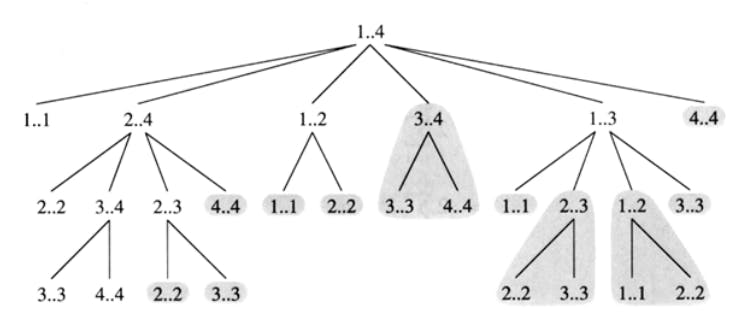
The other necessary property is overlapping sub-problems. A problem is said to have overlapping sub-problem properties if the sub-problems can be seen recursively visiting the same sub-problems. In such cases, we can improve the performance of an algorithm by storing the results of each sub-problem once it is calculated.

Dynamic Programming Techniques

There are two dynamic programming methods of implementation.

Top-Down Approach

This approach solves the bigger problem by recursively solving smaller sub-problems. As we solve the sub-problems, we store the result for later use. This way, we don’t need to solve the same sub-problem more than once. This method of saving the intermediate results is called Memoization.

Bottom-Up Approach

The bottom-up method is an iterative version of the top-down approach. This approach starts with the smallest and works upwards to the largest sub-problems. Thus when solving a particular sub-problem, we already have results of smaller dependent sub-problems. The results are stored in an n-dimensional (n=>0) table. Thus, you can imagine when we arrive at the original problem, we have solved all its sub-problems. Now we just use the result set to find the best solution. This method is called Tabulation.

EXAMPLE PROBLEM

You are climbing a staircase. It takes n steps to reach the top. Each time you can either climb 1 or 2 steps. In how many distinct ways can you climb to the top?

Input: n = 2
Output: 2
Explanation: There are two ways to climb to the top.
1. 1 step + 1 step
2. 2 steps

Implementation

We'll explore multiple approaches from simple to more complex, incrementally improving upon each solution.

1. Naive recursion

We can translate the recurrence we came up with earlier into code, as follows:

class Solution:
    def climbStairs(self, n: int) -> int:
        if n == 1:
            return 1
        if n == 2:
            return 2
        else:
            return self.climbStairs(n - 1) + self.climbStairs(n - 2)

However, running this yields Time Limit Exceeded. Why is it so inefficient? Let's think about calculating the ways to climb 6 stairs, climbStairs(6).

  climbStairs(6)
                                     /               \
                                cS(5)       +          cS(4)
                               /    \                  /    \
                           cS(4)   +   cS(3)         cS(3) + cS(2)
                           /  \        /   \         /   \
                      cS(3) + cS(2) cS(2) + cS(1) cS(2) + cS(1)
                      /  \
                 cS(2) + cS(1)

As you can see from the recursion tree above, we are calculating climbStairs(4) and climbStairs(3) multiple times. Specifically, climbStairs(4) is being recalculated twice, while climbStairs(3) is being recalculated 3 times. If you think about what happens for larger values of n, you can see that we are recalculating a lot of values!

Complexity

• Time: Each additional level in the recursion tree is going to have double the amount of calls to climbingStairs than the one above it. For n, this gives us a staggering 2^n function calls, for a O(2^n) time complexity. No wonder we get TLE!

• Space: We aren't storing any additional variables, so that's a O(1) space complexity.

Can we avoid repeated computation? Yes we can with the Top-Down DP.

2. Memoization (Top-Down DP)

What if instead of recomputing each value of climbStairs, we made sure to save the unique values (such as climbingStairs(5)), trading space for time? That's what a top-down dynamic programming approach called memoization is. We make use of a dictionary memo in which we store the values of climbStairs that we have computed, and if we ever have to compute that value again we just check memo in (average) O(1) time instead of doing the work all over again.

class Solution:
    def climbStairs(self, n: int) -> int:
        def climb(n):  # inner function to make code simpler
            if n in memo:
                return memo[n]
            else:
                memo[n] = climb(n-1) + climb(n-2)
                return memo[n]
        memo = {1: 1, 2: 2}  # base cases
        return climb(n)

This top-down paradigm works well when we approach the problem from the top of the stairs (the last step we needed to climb, n) down.

Complexity

• Time: There are O(n) distinct subproblems to solve, each requiring only O(1) amount of work of getting the values of smaller subproblems from memo and adding them together. When we encounter a subproblem we've already solved, we can get the answer in O(1) time.

• Space: We are using an additional memo dictionary that will store the answer to each subproblem, so O(n) space complexity.

Can we be even more efficient and avoid the overhead of recursion? Yes , with the help of Bottom-Up DP.

3. Bottom-Up DP
Turns out we can build the solution from the ground up (quite literally in this case). From our recurrence relation, we saw that the number of ways to climb n stairs depends on the number of ways to climb n - 1 and n - 2 stairs. So instead of approaching the problem top-down and computing these values recursively, we compute them bottom-up, starting with the base cases and building upon the previous values until we reach n. We use a dp array of length n + 1 (to accomodate for the 0-based indexing of Python; we could just have it be length n and return dp[n - 1] but in this way we are aligning the step numbers with the indices) and successively build up each index from the previous two.

class Solution:
    def climbStairs(self, n: int) -> int:
        if n == 1 or n == 2:
            return n
        dp = [-1] * (n + 1)  # to accomodate for 0-based indexing 
        dp[1], dp[2] = 1, 2
        for i in range(3, n + 1):
            dp[i] = dp[i - 1] + dp[i - 2]
        return dp[n]

Complexity

• Time: As before, we are computing each subproblem once and each subproblem requires constant amount of work (just the addition of the previous 2 elements of the array). That's O(n) time complexity.

• Space: Since we are storing the answers to previous subproblems in the dp array, this will be O(n) too.

• We can optimize one more time with the space optimization by maintaing just variables instead of storing the data in an array.

• Optimizied Bottom-Up DP
  While the above works well enough, we can optimize our approach even further by making a simple but important observation: we are only utilizing the last 2 subproblem answers when solving each subproblem. If you look at the recurrence again, you can see that the only pieces information we use are ways(n - 1) and ways(n - 2). Since we're computing from bottom-up, once we compute those answers, the smaller subproblems (such as ways(n - 3)) are not needed anymore. Thus, instead of keeping the entire dp array, we can save some space and just maintain 2 variables that track our last 2 subproblem answers!

•         class Solution:
              def climbStairs(self, n: int) -> int:
                  if n <= 2:
                      return n
                  ways = 0
                  # base cases
                  two_below_curr = 1  # 2 steps below 3 - ways to take 1 step: 1
                  one_below_curr = 2  # 1 step below 3 - ways to take 2 steps: 2
                  for i in range(3, n + 1):
                      # compute number of ways for i
                      ways = one_below_curr + two_below_curr
                      # step up to i + 1   
                      # 1 step below becomes 2 steps below
                      # current number of ways becomes 1 step below
                      two_below_curr, one_below_curr = one_below_curr, ways
  
                  return ways
  

  Complexity:

  • Time: As before, we are computing each subproblem once and each subproblem requires constant amount of work (just the addition of the previous 2 number of ways). That's O(n) time complexity.

  • Space: O(1) since we are maintaining 3 extra variables only!

And that's it! With using Dynamic Programming we went from a TLE solution to an elegant and optimized version.

Conclusion

One might find dynamic programming a bit intimidating initially. But if one understands the basics well, one can master dynamic programming problems. Having a strong programming foundation is key to getting comfortable with such problems. Applications of dynamic programming are common and relevant to everyday challenges, and mastering dynamic programming gives you the superpower to tacproachkle them.